W#02 Data Visualization Data Formats
Part 2 - A tour with code
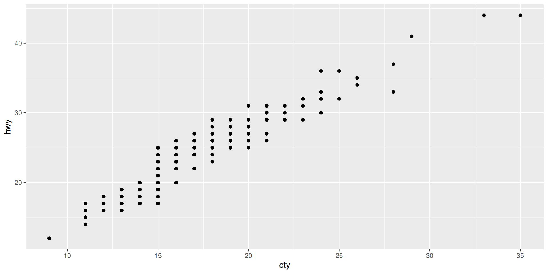
First plot in a basic specification
We take cty = “city miles per gallon” as x and hwy = “highway miles per gallon” as y

Compare to “The complete template” from the cheat sheet
It has all the required elements: We specify the data in the ggplot command, and the aesthetics (what variable is x and what variable is y) as mapping in the geom-function.
It also works this way

- In principle, we can specify new data and aesthetics in each geom-function in the same ggplot! Usually, we only have one dataset and one specification of aesthetics
And also this way

Even shorter
As common practice we can shorten the code and remove the data = and the mapping = because the first argument will be taken as data (if not specified otherwise) and the second as mapping (if not specified otherwise). See function documentation ?ggplot
The shortest
We can even remove the “x =” and “y =” if we look at the specification of aes() in ?aes

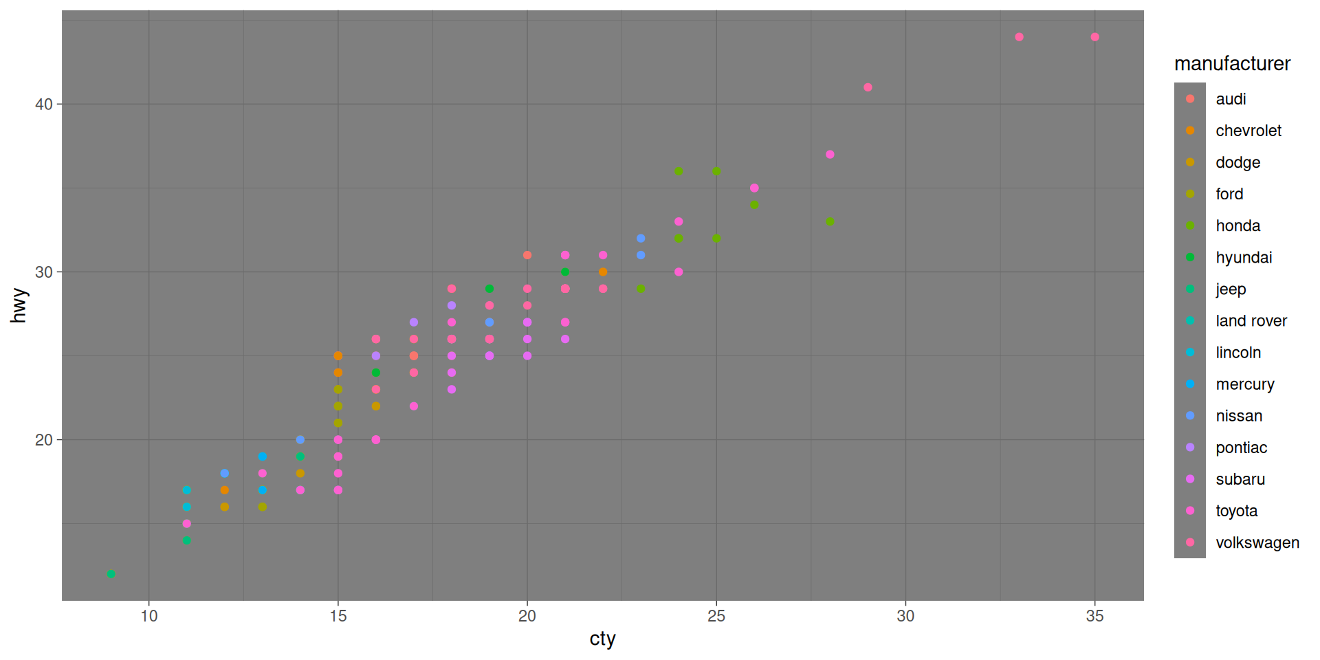
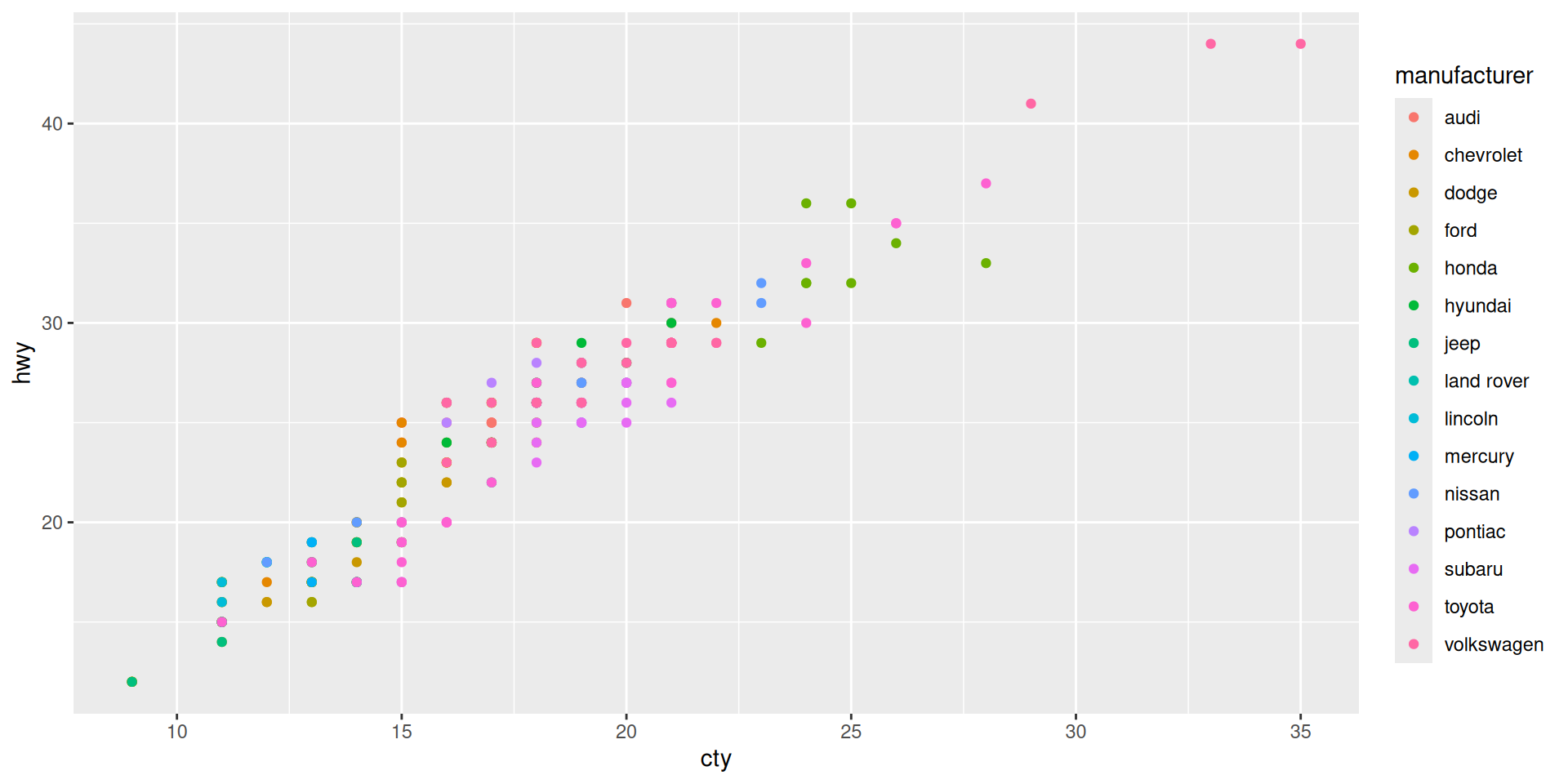
More aesthetics
color, shape, size, fill …
These need to be specified by name and cannot be left out.
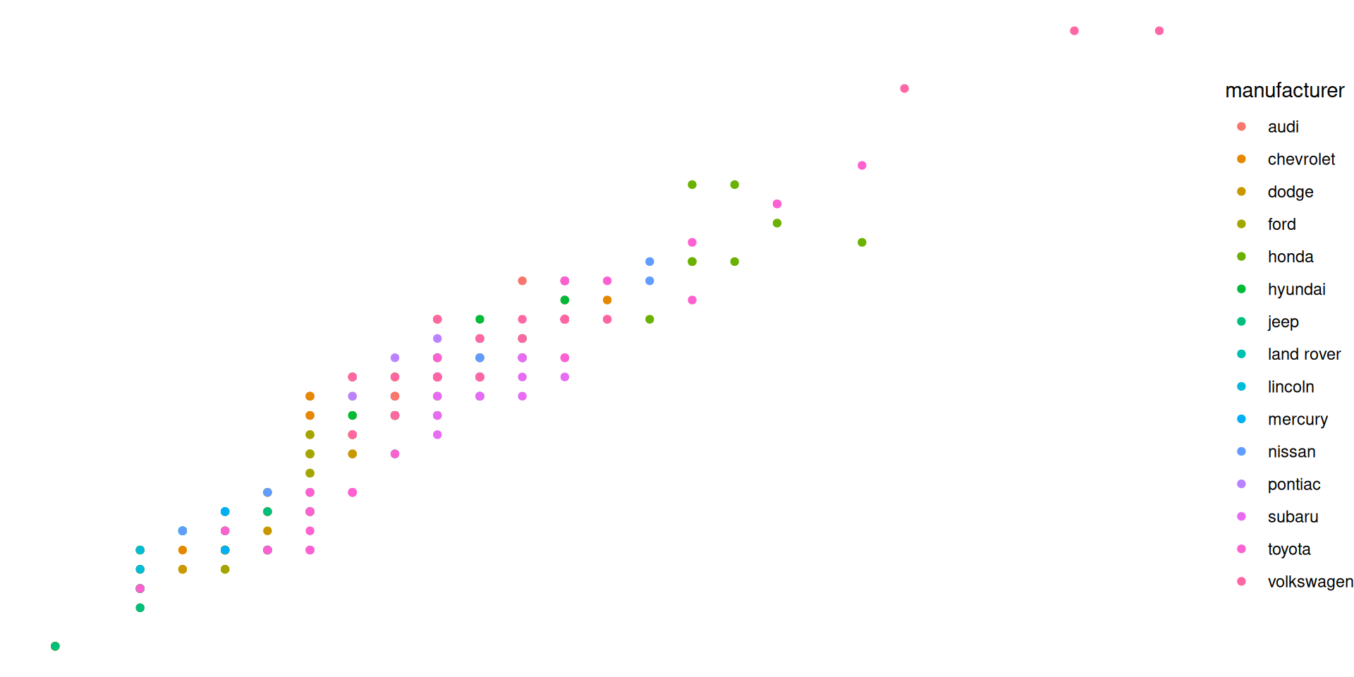
Let us color the manufacturer, and make size by cylinders
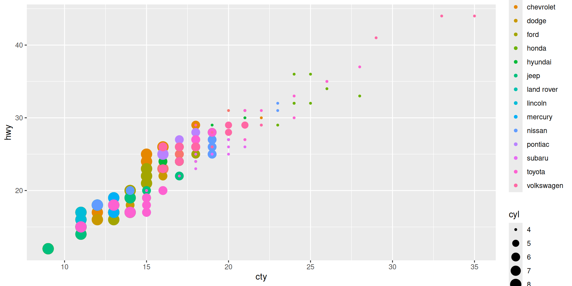
Do you like the plot?
Some critique:
- Too many colors
- Looks like several points are in the same place but we do not see it.
- Sizes look “unproportional” (4 is too small)

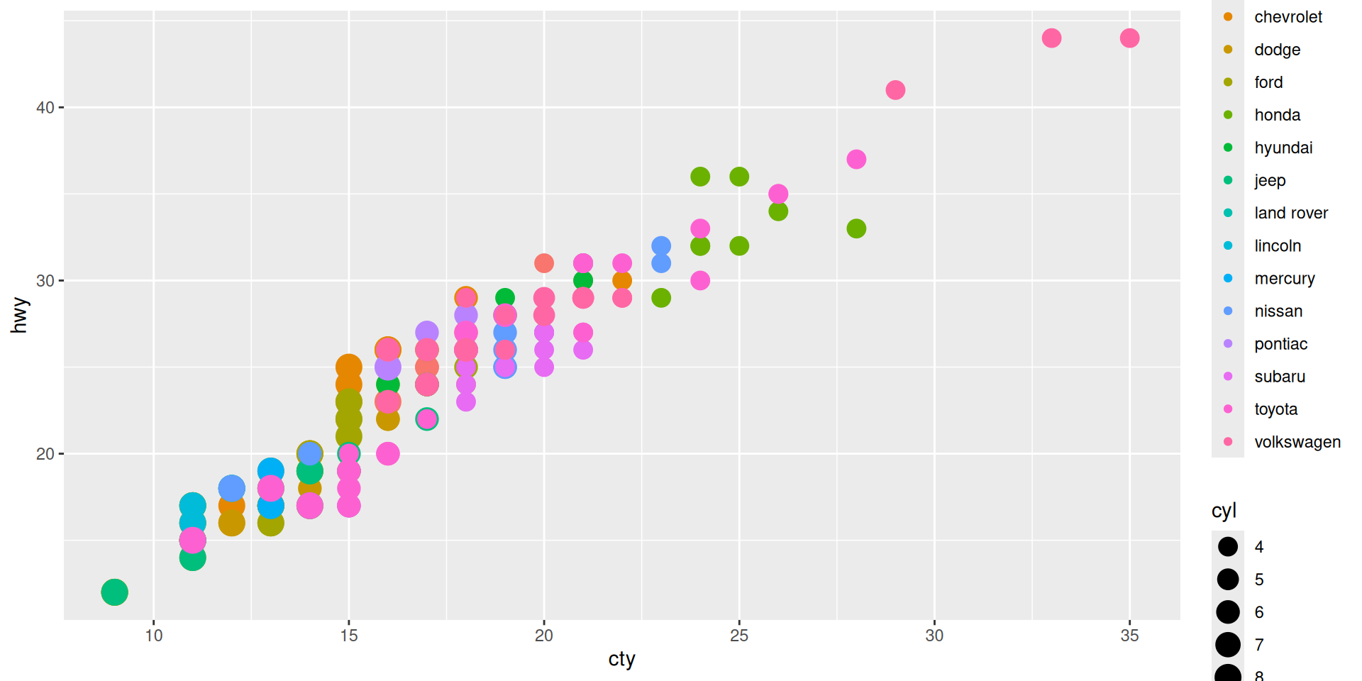
Work with scale_... to modify aesthetic’s look
Example: Scale the size differently
Check overplotting with a jitter
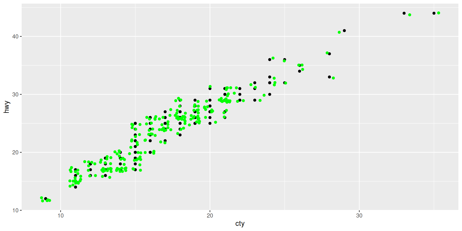
Here, we do two new things:
- We added another geom-function to an existing one. That is a core idea of the grammar of graphics. (However, for a final version, we would probably not do geom_point together with geom_jitter.)
- We specify the color by a word. Important: This is not within an
aes()command!
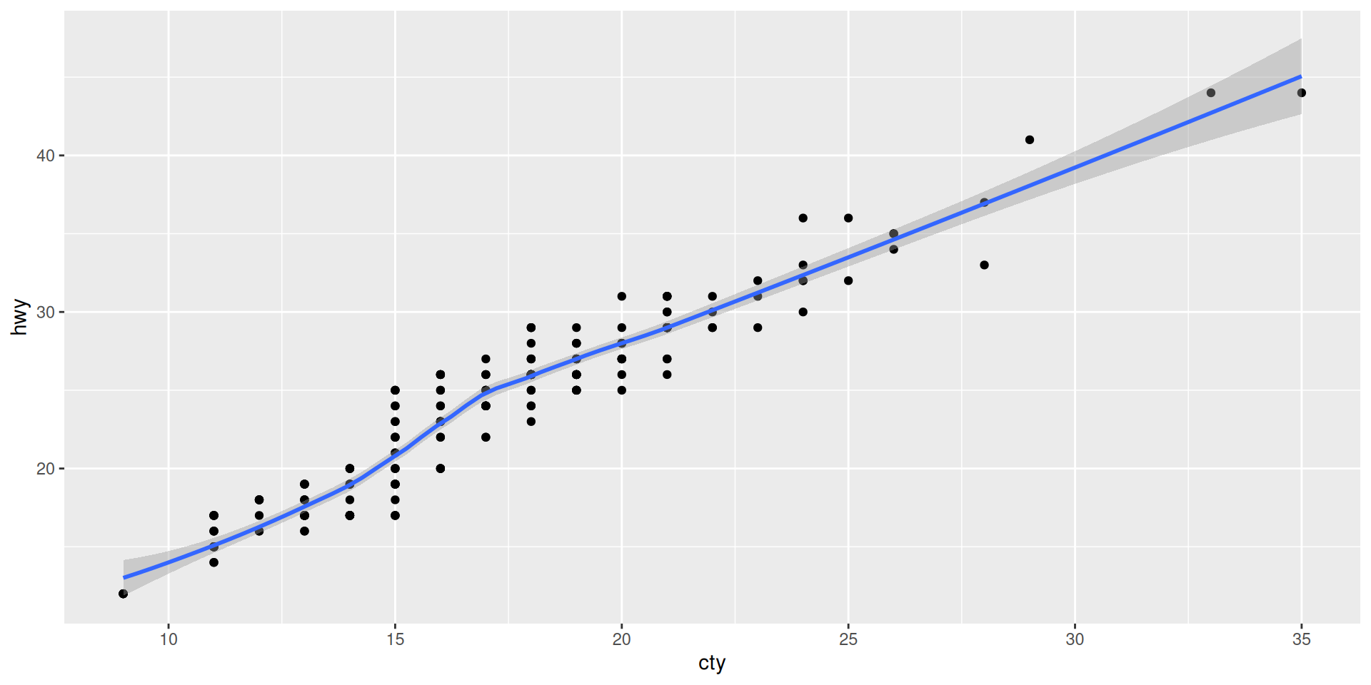
Another example for two geoms
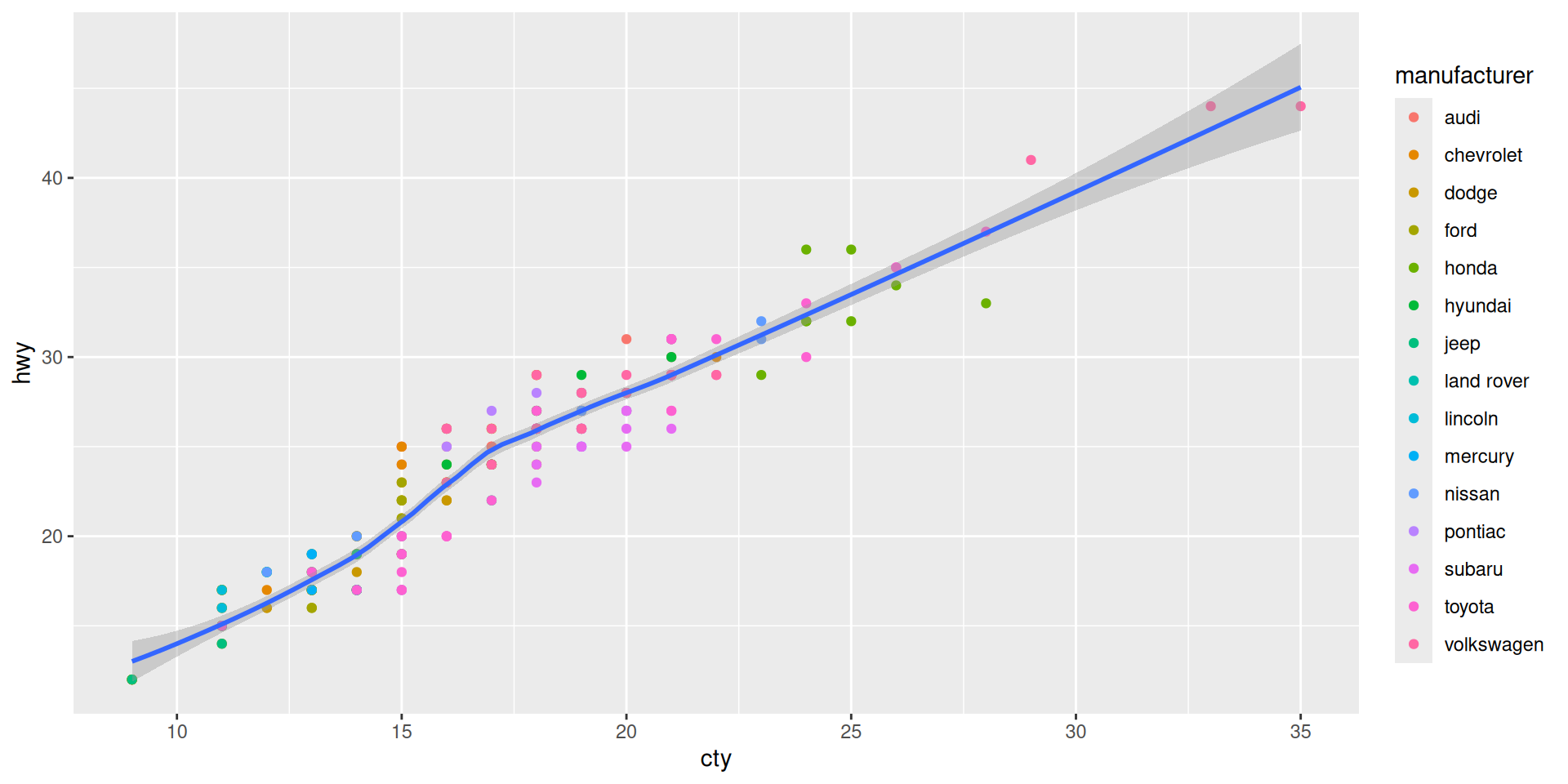
Add a smooth line as summary statistic
PUZZLE
What happens here? Why does green become red???
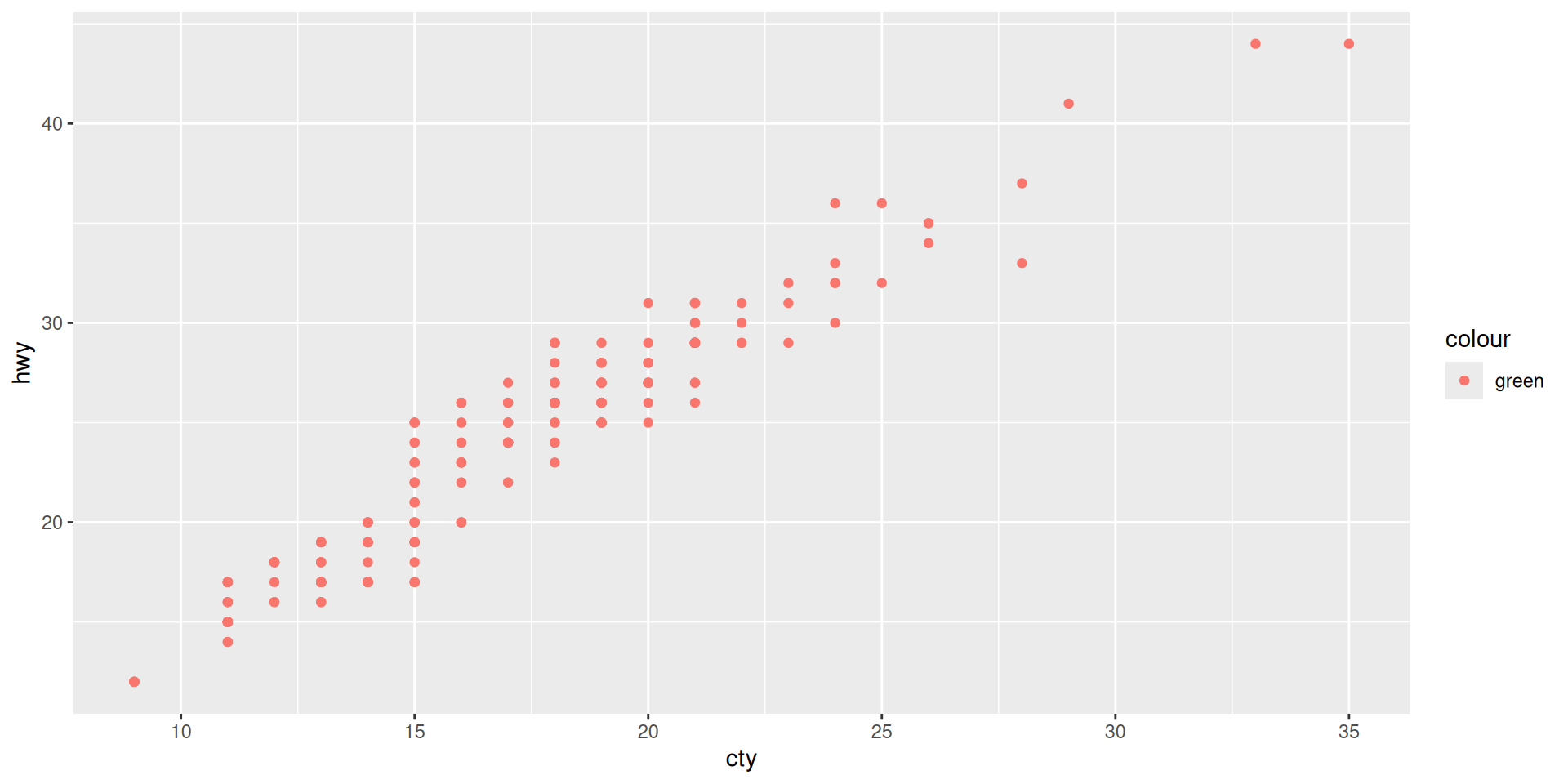
This is because “green” is taken here as a variable (with only one value for all data points).
So, “green” is not a color but a string and ggplot chooses color automatically.
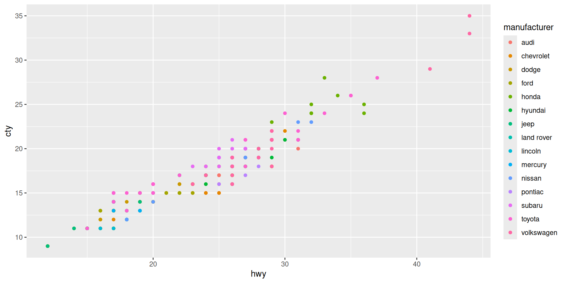
Call the object
As with other objects, when we write it in the console as such it provides an answer. In the case of ggplot-objects the answer is not some printed text in the console but a graphic output.
ggplot-Objects altered by more “+…”
Example
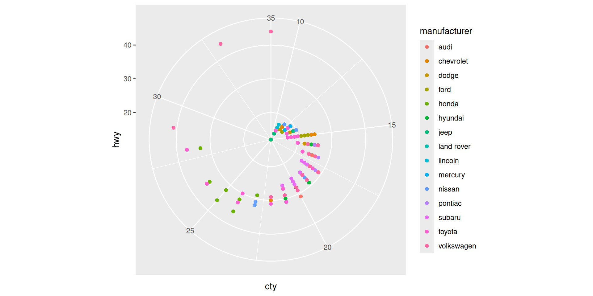
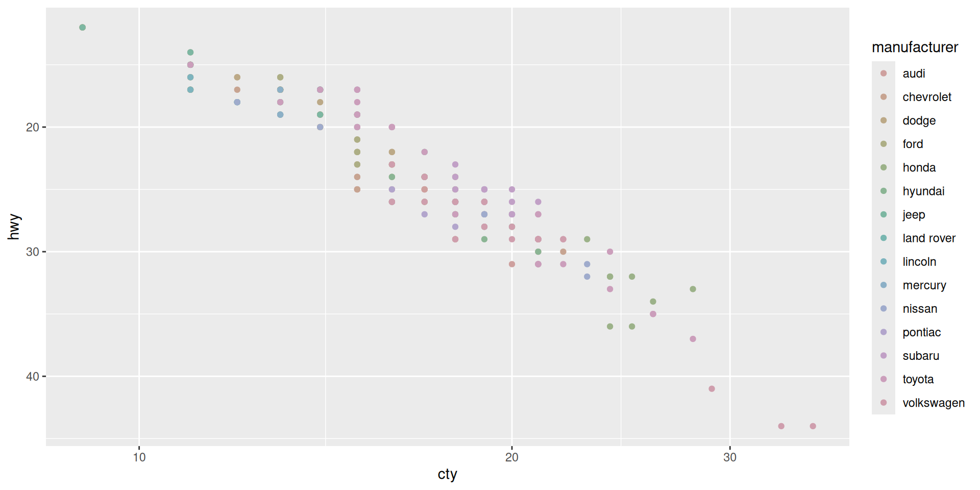
Coordinate system specification
Example
Coordinate system specification
Example
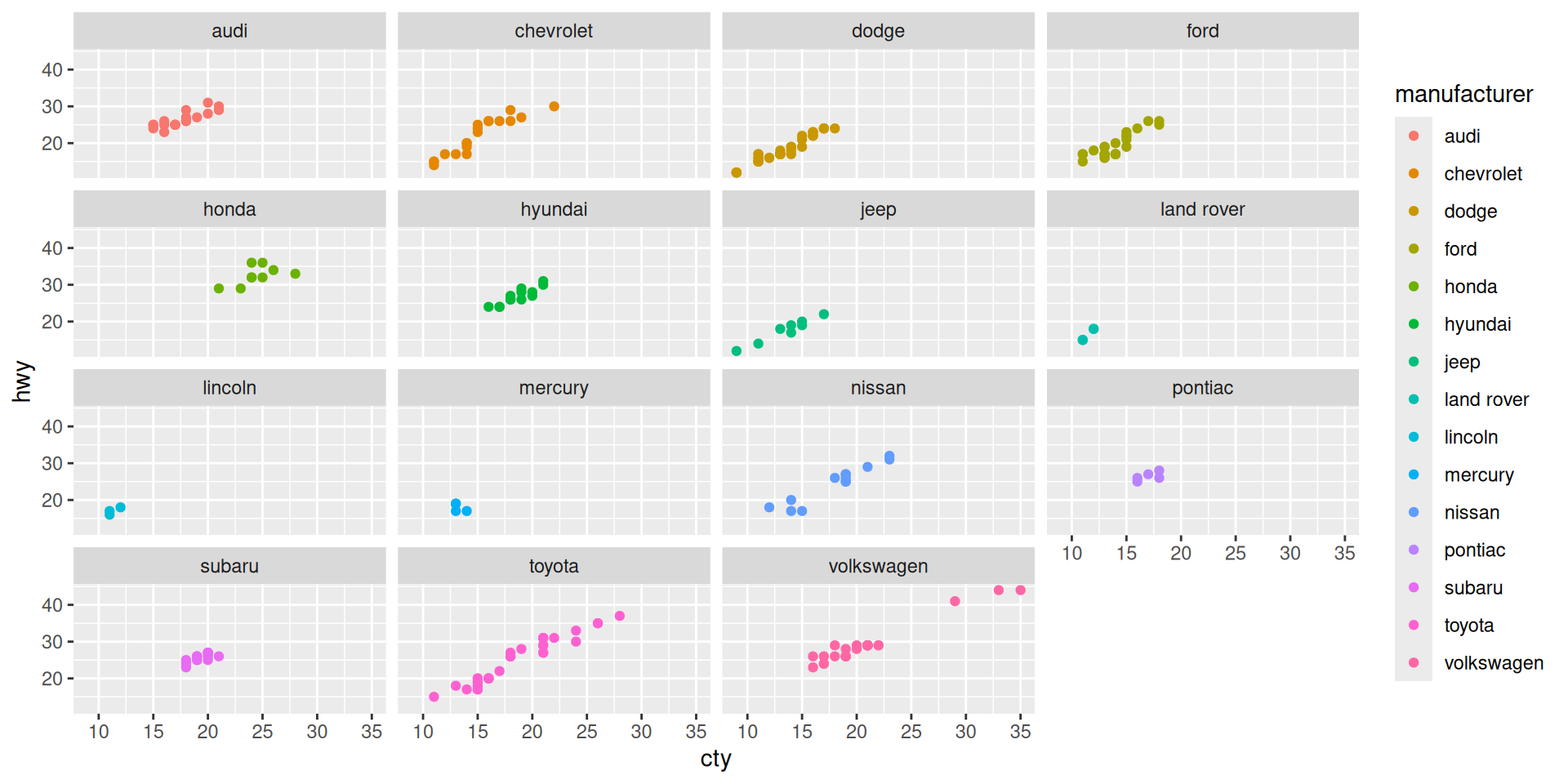
Faceting based on another variable
Example
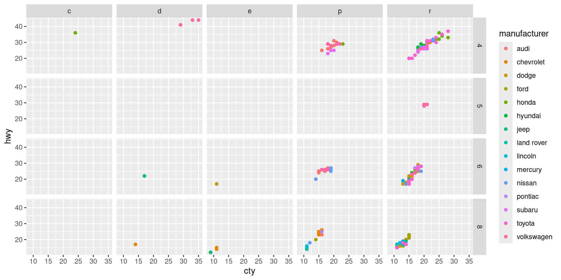
Faceting based on two other variables
Example
Scaling
Example
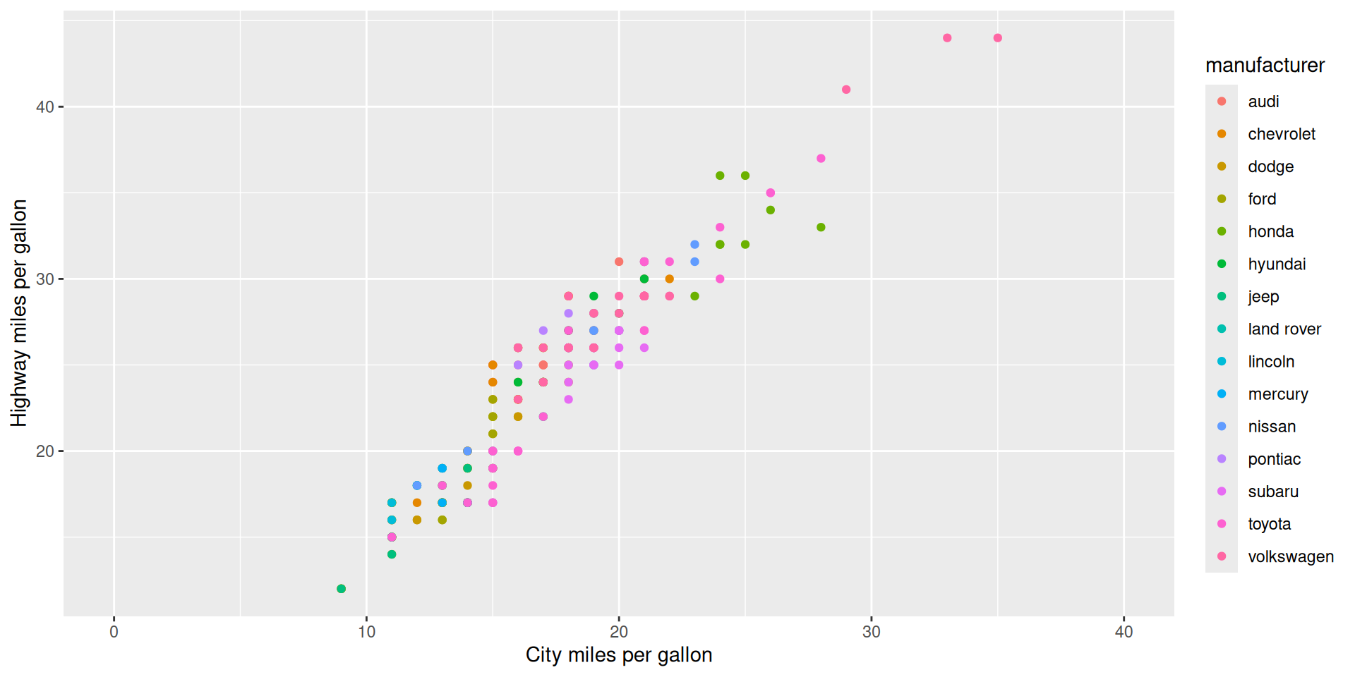
Axis limits and labels
Example
Themes
Example
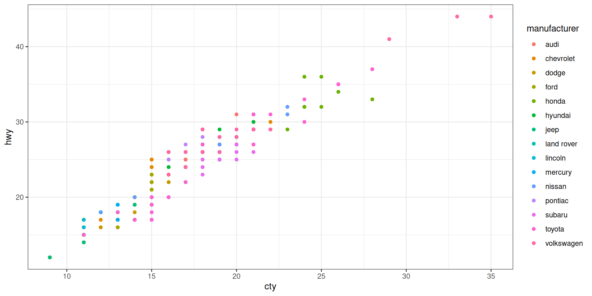
Themes
Example
Themes
Example